> ## Documentation Index
> Fetch the complete documentation index at: https://docs.pinecone.io/llms.txt
> Use this file to discover all available pages before exploring further.
# Cohere
> Connect Pinecone and Cohere to ship vector search and RAG applications: generate Cohere embeddings, index them in Pinecone, and rerank results.
export const PrimarySecondaryCTA = ({primaryLabel, primaryHref, primaryTarget, secondaryLabel, secondaryHref, secondaryTarget}) =>
{primaryLabel && primaryHref &&
}
{secondaryLabel && secondaryHref &&
}
 ### Set up the environment
Start by installing the Cohere and Pinecone clients and HuggingFace *Datasets* for downloading the TREC dataset used in this guide:
```shell Shell theme={null}
pip install -U cohere pinecone datasets
```
### Create embeddings
Sign up for an API key at [Cohere](https://dashboard.cohere.com/api-keys) and then use it to initialize your connection.
```Python Python theme={null}
import cohere
co = cohere.Client("")
```
Load the **T**ext **RE**trieval **C**onference (TREC) question classification dataset, which contains 5.5K labeled questions. You will take only the first 1K samples for this walkthrough, but this can be scaled to millions or even billions of samples.
```Python Python theme={null}
from datasets import load_dataset
# load the first 1K rows of the TREC dataset
trec = load_dataset('trec', split='train[:1000]')
```
Each sample in `trec` contains two label features and the *text* feature. Pass the questions from the *text* feature to Cohere to create embeddings.
```Python Python theme={null}
embeds = co.embed(
texts=trec['text'],
model='embed-english-v3.0',
input_type='search_document',
truncate='END'
).embeddings
```
Check the dimensionality of the returned vectors. You will need to save the embedding dimensionality from this to be used when initializing your Pinecone index later
```Python Python theme={null}
import numpy as np
shape = np.array(embeds).shape
print(shape)
# [Out]:
# (1000, 1024)
```
You can see the `1024` embedding dimensionality produced by Cohere's `embed-english-v3.0` model, and the `1000` samples you built embeddings for.
### Store the Embeddings
Now that you have your embeddings, you can move on to indexing them in the Pinecone vector database. For this, you need a [Pinecone API key](/guides/projects/manage-api-keys).
You first initialize our connection to Pinecone and then create a new index called `cohere-pinecone-trec` for storing the embeddings. When creating the index, you specify that you would like to use the cosine similarity metric to align with Cohere's embeddings, and also pass the embedding dimensionality of `1024`.
```Python Python theme={null}
from pinecone import Pinecone
# initialize connection to pinecone (get API key at app.pinecone.io)
pc = Pinecone(api_key='YOUR_API_KEY')
index_name = 'cohere-pinecone-trec'
# if the index does not exist, we create it
if not pc.has_index(index_name):
pc.create_index(
name=index_name,
dimension=shape[1],
metric="cosine",
spec=ServerlessSpec(
cloud='aws',
region='us-east-1'
)
)
# connect to index
index = pc.Index(index_name)
```
Now you can begin populating the index with your embeddings. Pinecone expects you to provide a list of tuples in the format *(id, vector, metadata)*, where the *metadata* field is an optional extra field where you can store anything you want in a dictionary format. For this example, you will store the original text of the embeddings.
While uploading your data, you will batch everything to avoid pushing too much data in one go.
```Python Python theme={null}
batch_size = 128
ids = [str(i) for i in range(shape[0])]
# create list of metadata dictionaries
meta = [{'text': text} for text in trec['text']]
# create list of (id, vector, metadata) tuples to be upserted
to_upsert = list(zip(ids, embeds, meta))
for i in range(0, shape[0], batch_size):
i_end = min(i+batch_size, shape[0])
index.upsert(vectors=to_upsert[i:i_end])
# let's view the index statistics
print(index.describe_index_stats())
# [Out]:
# {'dimension': 1024,
# 'index_fullness': 0.0,
# 'namespaces': {'': {'vector_count': 1000}},
# 'total_vector_count': 1000}
```
You can see from `index.describe_index_stats` that you have a *1024-dimensionality* index populated with *1000* embeddings. For serverless on-demand indexes, the `index_fullness` metric is typically `0` because storage and compute scale automatically. If you're using [dedicated read nodes](/guides/index-data/dedicated-read-nodes/concepts#index-fullness), `index_fullness` (along with `memory_fullness` and `storage_fullness`) tells you how close the index is to its allocated capacity.
### Semantic search
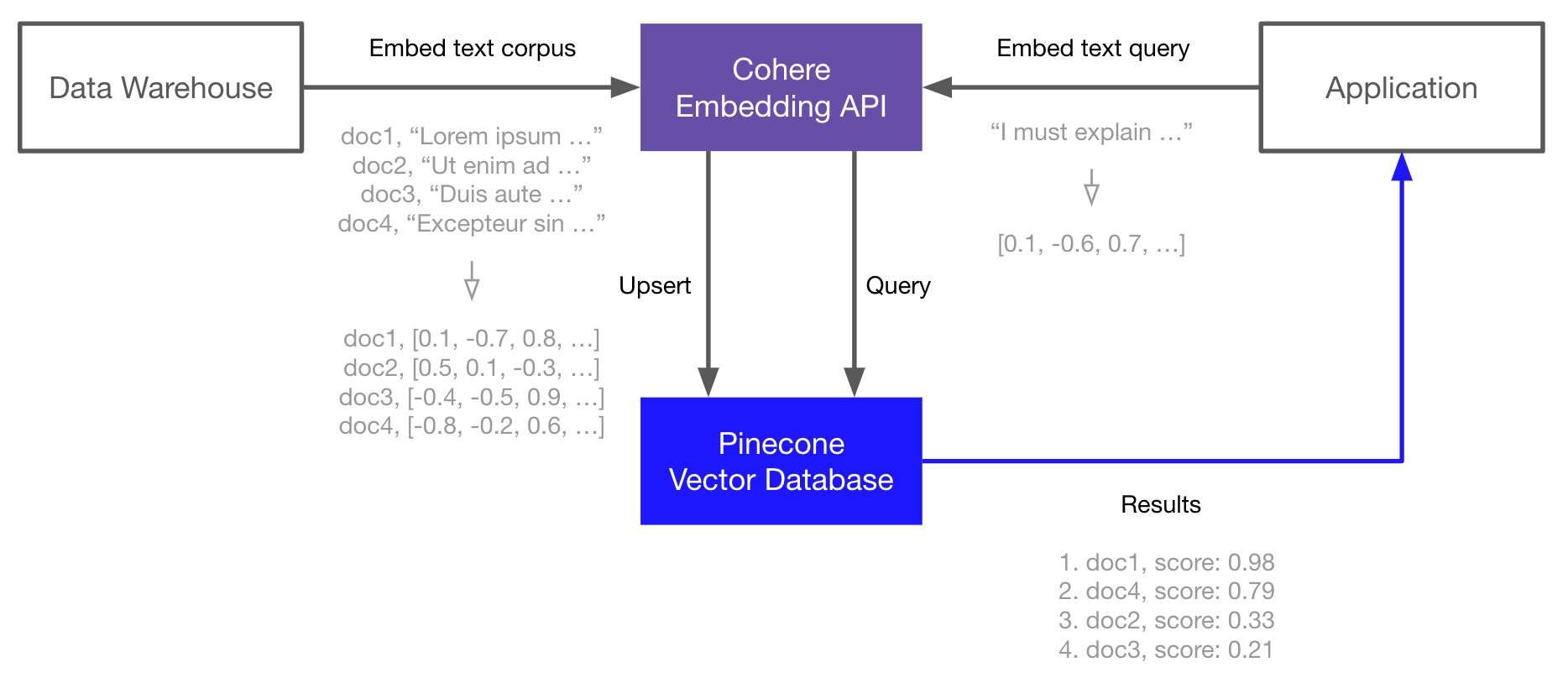
Now that you have your indexed vectors, you can perform a few search queries. When searching, you will first embed your query using Cohere, and then search using the returned vector in Pinecone.
```Python Python theme={null}
query = "What caused the 1929 Great Depression?"
# create the query embedding
xq = co.embed(
texts=[query],
model='embed-english-v3.0',
input_type='search_query',
truncate='END'
).embeddings
print(np.array(xq).shape)
# query, returning the top 5 most similar results
res = index.query(vector=xq, top_k=5, include_metadata=True)
```
The response from Pinecone includes your original text in the `metadata` field. Let's print out the `top_k` most similar questions and their respective similarity scores.
```Python Python theme={null}
for match in res['matches']:
print(f"{match['score']:.2f}: {match['metadata']['text']}")
# [Out]:
# 0.62: Why did the world enter a global depression in 1929 ?
# 0.49: When was `` the Great Depression '' ?
# 0.38: What crop failure caused the Irish Famine ?
# 0.32: What caused Harry Houdini 's death ?
# 0.31: What causes pneumonia ?
```
Looks good! Let's make it harder and replace *"depression"* with the incorrect term *"recession"*.
```Python Python theme={null}
query = "What was the cause of the major recession in the early 20th century?"
# create the query embedding
xq = co.embed(
texts=[query],
model='embed-english-v3.0',
input_type='search_query',
truncate='END'
).embeddings
# query, returning the top 5 most similar results
res = index.query(vector=xq, top_k=5, include_metadata=True)
for match in res['matches']:
print(f"{match['score']:.2f}: {match['metadata']['text']}")
# [Out]:
# 0.43: When was `` the Great Depression '' ?
# 0.40: Why did the world enter a global depression in 1929 ?
# 0.39: When did World War I start ?
# 0.35: What are some of the significant historical events of the 1990s ?
# 0.32: What crop failure caused the Irish Famine ?
```
Let's perform one final search using the definition of depression rather than the word or related words.
```Python Python theme={null}
query = "Why was there a long-term economic downturn in the early 20th century?"
# create the query embedding
xq = co.embed(
texts=[query],
model='embed-english-v3.0',
input_type='search_query',
truncate='END'
).embeddings
# query, returning the top 10 most similar results
res = index.query(vector=xq, top_k=10, include_metadata=True)
for match in res['matches']:
print(f"{match['score']:.2f}: {match['metadata']['text']}")
# [Out]:
# 0.40: When was `` the Great Depression '' ?
# 0.39: Why did the world enter a global depression in 1929 ?
# 0.35: When did World War I start ?
# 0.32: What are some of the significant historical events of the 1990s ?
# 0.31: What war did the Wanna-Go-Home Riots occur after ?
# 0.31: What do economists do ?
# 0.29: What historical event happened in Dogtown in 1899 ?
# 0.28: When did the Dow first reach ?
# 0.28: Who earns their money the hard way ?
# 0.28: What were popular songs and types of songs in the 1920s ?
```
It's clear from this example that the semantic search pipeline is clearly able to identify the meaning between each of your queries. Using these embeddings with Pinecone allows you to return the most semantically similar questions from the already indexed TREC dataset.
### Set up the environment
Start by installing the Cohere and Pinecone clients and HuggingFace *Datasets* for downloading the TREC dataset used in this guide:
```shell Shell theme={null}
pip install -U cohere pinecone datasets
```
### Create embeddings
Sign up for an API key at [Cohere](https://dashboard.cohere.com/api-keys) and then use it to initialize your connection.
```Python Python theme={null}
import cohere
co = cohere.Client("")
```
Load the **T**ext **RE**trieval **C**onference (TREC) question classification dataset, which contains 5.5K labeled questions. You will take only the first 1K samples for this walkthrough, but this can be scaled to millions or even billions of samples.
```Python Python theme={null}
from datasets import load_dataset
# load the first 1K rows of the TREC dataset
trec = load_dataset('trec', split='train[:1000]')
```
Each sample in `trec` contains two label features and the *text* feature. Pass the questions from the *text* feature to Cohere to create embeddings.
```Python Python theme={null}
embeds = co.embed(
texts=trec['text'],
model='embed-english-v3.0',
input_type='search_document',
truncate='END'
).embeddings
```
Check the dimensionality of the returned vectors. You will need to save the embedding dimensionality from this to be used when initializing your Pinecone index later
```Python Python theme={null}
import numpy as np
shape = np.array(embeds).shape
print(shape)
# [Out]:
# (1000, 1024)
```
You can see the `1024` embedding dimensionality produced by Cohere's `embed-english-v3.0` model, and the `1000` samples you built embeddings for.
### Store the Embeddings
Now that you have your embeddings, you can move on to indexing them in the Pinecone vector database. For this, you need a [Pinecone API key](/guides/projects/manage-api-keys).
You first initialize our connection to Pinecone and then create a new index called `cohere-pinecone-trec` for storing the embeddings. When creating the index, you specify that you would like to use the cosine similarity metric to align with Cohere's embeddings, and also pass the embedding dimensionality of `1024`.
```Python Python theme={null}
from pinecone import Pinecone
# initialize connection to pinecone (get API key at app.pinecone.io)
pc = Pinecone(api_key='YOUR_API_KEY')
index_name = 'cohere-pinecone-trec'
# if the index does not exist, we create it
if not pc.has_index(index_name):
pc.create_index(
name=index_name,
dimension=shape[1],
metric="cosine",
spec=ServerlessSpec(
cloud='aws',
region='us-east-1'
)
)
# connect to index
index = pc.Index(index_name)
```
Now you can begin populating the index with your embeddings. Pinecone expects you to provide a list of tuples in the format *(id, vector, metadata)*, where the *metadata* field is an optional extra field where you can store anything you want in a dictionary format. For this example, you will store the original text of the embeddings.
While uploading your data, you will batch everything to avoid pushing too much data in one go.
```Python Python theme={null}
batch_size = 128
ids = [str(i) for i in range(shape[0])]
# create list of metadata dictionaries
meta = [{'text': text} for text in trec['text']]
# create list of (id, vector, metadata) tuples to be upserted
to_upsert = list(zip(ids, embeds, meta))
for i in range(0, shape[0], batch_size):
i_end = min(i+batch_size, shape[0])
index.upsert(vectors=to_upsert[i:i_end])
# let's view the index statistics
print(index.describe_index_stats())
# [Out]:
# {'dimension': 1024,
# 'index_fullness': 0.0,
# 'namespaces': {'': {'vector_count': 1000}},
# 'total_vector_count': 1000}
```
You can see from `index.describe_index_stats` that you have a *1024-dimensionality* index populated with *1000* embeddings. For serverless on-demand indexes, the `index_fullness` metric is typically `0` because storage and compute scale automatically. If you're using [dedicated read nodes](/guides/index-data/dedicated-read-nodes/concepts#index-fullness), `index_fullness` (along with `memory_fullness` and `storage_fullness`) tells you how close the index is to its allocated capacity.
### Semantic search
Now that you have your indexed vectors, you can perform a few search queries. When searching, you will first embed your query using Cohere, and then search using the returned vector in Pinecone.
```Python Python theme={null}
query = "What caused the 1929 Great Depression?"
# create the query embedding
xq = co.embed(
texts=[query],
model='embed-english-v3.0',
input_type='search_query',
truncate='END'
).embeddings
print(np.array(xq).shape)
# query, returning the top 5 most similar results
res = index.query(vector=xq, top_k=5, include_metadata=True)
```
The response from Pinecone includes your original text in the `metadata` field. Let's print out the `top_k` most similar questions and their respective similarity scores.
```Python Python theme={null}
for match in res['matches']:
print(f"{match['score']:.2f}: {match['metadata']['text']}")
# [Out]:
# 0.62: Why did the world enter a global depression in 1929 ?
# 0.49: When was `` the Great Depression '' ?
# 0.38: What crop failure caused the Irish Famine ?
# 0.32: What caused Harry Houdini 's death ?
# 0.31: What causes pneumonia ?
```
Looks good! Let's make it harder and replace *"depression"* with the incorrect term *"recession"*.
```Python Python theme={null}
query = "What was the cause of the major recession in the early 20th century?"
# create the query embedding
xq = co.embed(
texts=[query],
model='embed-english-v3.0',
input_type='search_query',
truncate='END'
).embeddings
# query, returning the top 5 most similar results
res = index.query(vector=xq, top_k=5, include_metadata=True)
for match in res['matches']:
print(f"{match['score']:.2f}: {match['metadata']['text']}")
# [Out]:
# 0.43: When was `` the Great Depression '' ?
# 0.40: Why did the world enter a global depression in 1929 ?
# 0.39: When did World War I start ?
# 0.35: What are some of the significant historical events of the 1990s ?
# 0.32: What crop failure caused the Irish Famine ?
```
Let's perform one final search using the definition of depression rather than the word or related words.
```Python Python theme={null}
query = "Why was there a long-term economic downturn in the early 20th century?"
# create the query embedding
xq = co.embed(
texts=[query],
model='embed-english-v3.0',
input_type='search_query',
truncate='END'
).embeddings
# query, returning the top 10 most similar results
res = index.query(vector=xq, top_k=10, include_metadata=True)
for match in res['matches']:
print(f"{match['score']:.2f}: {match['metadata']['text']}")
# [Out]:
# 0.40: When was `` the Great Depression '' ?
# 0.39: Why did the world enter a global depression in 1929 ?
# 0.35: When did World War I start ?
# 0.32: What are some of the significant historical events of the 1990s ?
# 0.31: What war did the Wanna-Go-Home Riots occur after ?
# 0.31: What do economists do ?
# 0.29: What historical event happened in Dogtown in 1899 ?
# 0.28: When did the Dow first reach ?
# 0.28: Who earns their money the hard way ?
# 0.28: What were popular songs and types of songs in the 1920s ?
```
It's clear from this example that the semantic search pipeline is clearly able to identify the meaning between each of your queries. Using these embeddings with Pinecone allows you to return the most semantically similar questions from the already indexed TREC dataset.